tidymodels 1 recipes in R on hotel booking

1 package

Code

library(tidyverse)
library(ggplot2)
library(tidymodels)
library(rsample)
library(themis)

2 data

Code

library(tidyverse)

hotels <- readr::read_csv("https://raw.githubusercontent.com/rfordatascience/tidytuesday/master/data/2020/2020-02-11/hotels.csv")


hotel_stays <- hotels %>%
  filter(is_canceled == 0) %>%
  mutate(
    children = case_when(
      children + babies > 0 ~ "children",
      TRUE ~ "none"
    ),
    required_car_parking_spaces = case_when(
      required_car_parking_spaces > 0 ~ "parking",
      TRUE ~ "none"
    )
  ) %>%
  select(-is_canceled, -reservation_status, -babies)

hotel_stays

# A tibble: 75,166 × 29
   hotel   lead_time arrival_date_year arrival_date_month arrival_date_week_nu…¹
   <chr>       <dbl>             <dbl> <chr>                               <dbl>
 1 Resort…       342              2015 July                                   27
 2 Resort…       737              2015 July                                   27
 3 Resort…         7              2015 July                                   27
 4 Resort…        13              2015 July                                   27
 5 Resort…        14              2015 July                                   27
 6 Resort…        14              2015 July                                   27
 7 Resort…         0              2015 July                                   27
 8 Resort…         9              2015 July                                   27
 9 Resort…        35              2015 July                                   27
10 Resort…        68              2015 July                                   27
# ℹ 75,156 more rows
# ℹ abbreviated name: ¹​arrival_date_week_number
# ℹ 24 more variables: arrival_date_day_of_month <dbl>,
#   stays_in_weekend_nights <dbl>, stays_in_week_nights <dbl>, adults <dbl>,
#   children <chr>, meal <chr>, country <chr>, market_segment <chr>,
#   distribution_channel <chr>, is_repeated_guest <dbl>,
#   previous_cancellations <dbl>, previous_bookings_not_canceled <dbl>, …

2.1 EDA

Code

hotel_stays %>%
  count(children)

# A tibble: 2 × 2
  children     n
  <chr>    <int>
1 children  6073
2 none     69093

Code

library(skimr)

skim(hotel_stays)

Data summary

Name	hotel_stays
Number of rows	75166
Number of columns	29
_______________________
Column type frequency:
character	14
Date	1
numeric	14
________________________
Group variables	None

Variable type: character

skim_variable	n_missing	complete_rate	min	max	empty	n_unique	whitespace
hotel	0	1	10	12	0	2	0
arrival_date_month	0	1	3	9	0	12	0
children	0	1	4	8	0	2	0
meal	0	1	2	9	0	5	0
country	0	1	2	4	0	166	0
market_segment	0	1	6	13	0	7	0
distribution_channel	0	1	3	9	0	5	0
reserved_room_type	0	1	1	1	0	9	0
assigned_room_type	0	1	1	1	0	10	0
deposit_type	0	1	10	10	0	3	0
agent	0	1	1	4	0	315	0
company	0	1	1	4	0	332	0
customer_type	0	1	5	15	0	4	0
required_car_parking_spaces	0	1	4	7	0	2	0

Variable type: Date

skim_variable	n_missing	complete_rate	min	max	median	n_unique
reservation_status_date	0	1	2015-07-01	2017-09-14	2016-09-01	805

Variable type: numeric

skim_variable	n_missing	complete_rate	mean	sd	p0	p25	p50	p75	p100	hist
lead_time	0	1	79.98	91.11	0.00	9.0	45.0	124	737	▇▂▁▁▁
arrival_date_year	0	1	2016.15	0.70	2015.00	2016.0	2016.0	2017	2017	▃▁▇▁▆
arrival_date_week_number	0	1	27.08	13.90	1.00	16.0	28.0	38	53	▆▇▇▇▆
arrival_date_day_of_month	0	1	15.84	8.78	1.00	8.0	16.0	23	31	▇▇▇▇▆
stays_in_weekend_nights	0	1	0.93	0.99	0.00	0.0	1.0	2	19	▇▁▁▁▁
stays_in_week_nights	0	1	2.46	1.92	0.00	1.0	2.0	3	50	▇▁▁▁▁
adults	0	1	1.83	0.51	0.00	2.0	2.0	2	4	▁▂▇▁▁
is_repeated_guest	0	1	0.04	0.20	0.00	0.0	0.0	0	1	▇▁▁▁▁
previous_cancellations	0	1	0.02	0.27	0.00	0.0	0.0	0	13	▇▁▁▁▁
previous_bookings_not_canceled	0	1	0.20	1.81	0.00	0.0	0.0	0	72	▇▁▁▁▁
booking_changes	0	1	0.29	0.74	0.00	0.0	0.0	0	21	▇▁▁▁▁
days_in_waiting_list	0	1	1.59	14.78	0.00	0.0	0.0	0	379	▇▁▁▁▁
adr	0	1	99.99	49.21	-6.38	67.5	92.5	125	510	▇▆▁▁▁
total_of_special_requests	0	1	0.71	0.83	0.00	0.0	1.0	1	5	▇▁▁▁▁

Code

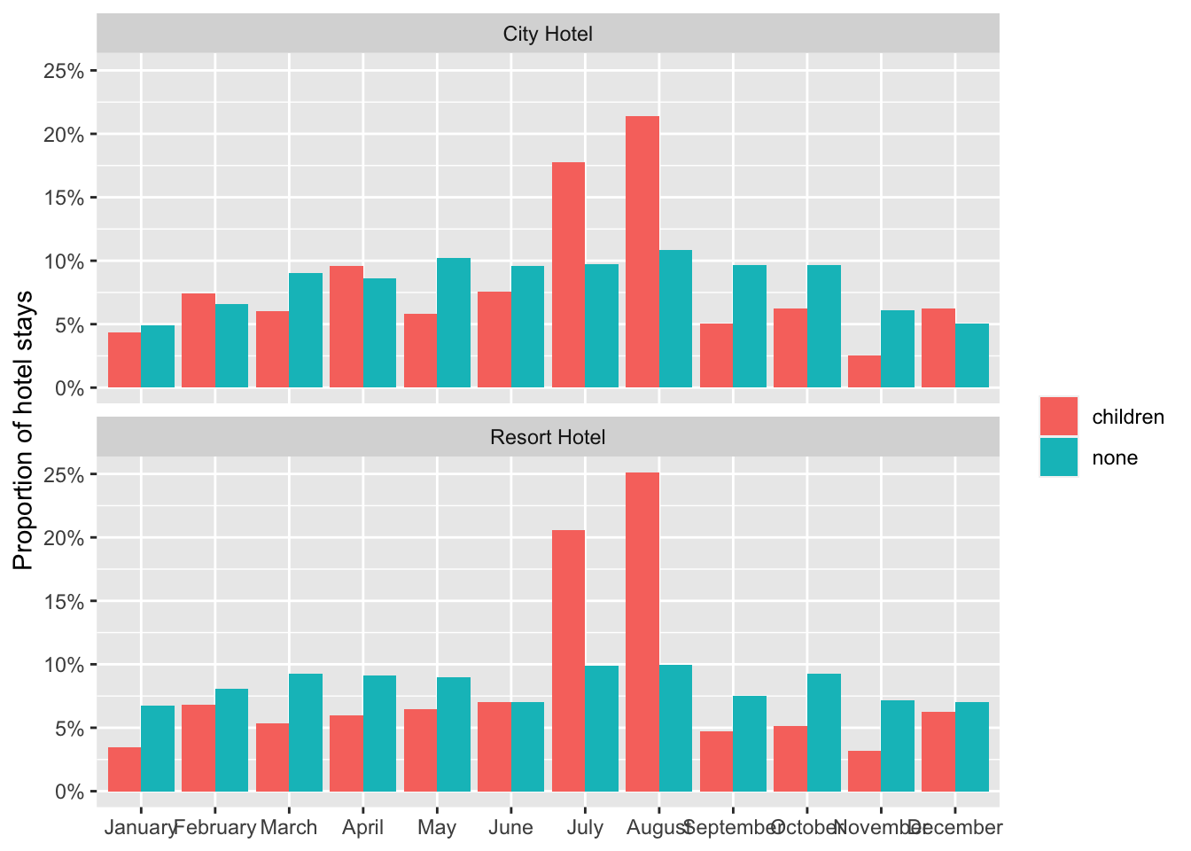
hotel_stays %>%
  mutate(arrival_date_month = factor(arrival_date_month,
    levels = month.name
  )) %>%
  count(hotel, arrival_date_month, children) %>%
  group_by(hotel, children) %>%
  mutate(proportion = n / sum(n)) %>%
  ggplot(aes(arrival_date_month, proportion, fill = children)) +
  geom_col(position = "dodge") +
  scale_y_continuous(labels = scales::percent_format()) +
  facet_wrap(~hotel, nrow = 2) +
  labs(
    x = NULL,
    y = "Proportion of hotel stays",
    fill = NULL
  )

2.2 data split

Code

hotels_df <- hotel_stays %>%
  select(
    children, hotel, arrival_date_month, meal, adr, adults,
    required_car_parking_spaces, total_of_special_requests,
    stays_in_week_nights, stays_in_weekend_nights
  ) %>%
  mutate_if(is.character, factor)

Code

library(tidymodels)

set.seed(1234)
hotel_split <- initial_split(hotels_df)

hotel_train <- training(hotel_split)
hotel_test <- testing(hotel_split)

3 model

3.1 recipe

Code

hotel_rec <- recipe(children ~ ., data = hotel_train) %>%
  step_downsample(children) %>%
  step_dummy(all_nominal(), -all_outcomes()) %>%
  step_zv(all_numeric()) %>%
  step_normalize(all_numeric()) %>%
  prep()

Difference on recipe();prep();bake();juice()

3.2 prep the recipe

Code

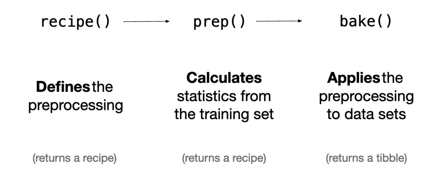
hotel_rec=hotel_rec %>% prep()

Code

hotel_rec

3.3 bake the train data with preded recipe

Code

train_proc <- bake(hotel_rec, new_data = hotel_train)

Code

train_proc2 <- bake(hotel_rec, new_data = NULL)

Code

train_juice <-juice(hotel_rec)

the difference between train_proc and train_juice is that the train_juice is been down sample.

Code

dim(train_proc)

[1] 56374    23

Code

dim(train_proc2)

[1] 9032   23

Code

dim(train_juice)

[1] 9032   23

Code

train_proc %>%
  count(children)

# A tibble: 2 × 2
  children     n
  <fct>    <int>
1 children  4516
2 none     51858

the juice and train_proc2 target is down sample to 1:1

Code

train_proc2 %>%
  count(children)

# A tibble: 2 × 2
  children     n
  <fct>    <int>
1 children  4516
2 none      4516

Code

train_juice %>%
  count(children)

# A tibble: 2 × 2
  children     n
  <fct>    <int>
1 children  4516
2 none      4516

3.4 bake the test data with preded recipe

Code

test_proc <- bake(hotel_rec, new_data = hotel_test)

juice(pre_recipe,data=NULL) is same as bake(pre_recipe,data=hotel_train) for training data (excepted down sample)

3.5 model

3.5.1 KNN model

Code

knn_spec <- nearest_neighbor() %>%
  set_engine("kknn") %>%
  set_mode("classification")

3.5.2 tree model

Code

tree_spec <- decision_tree() %>%
  set_engine("rpart") %>%
  set_mode("classification")

3.6 workflow

not using workflow in this case

3.7 training

training with train data(baked).

Code

knn_fit <- knn_spec %>%
  fit(children ~ ., data = train_juice)

knn_fit

parsnip model object


Call:
kknn::train.kknn(formula = children ~ ., data = data, ks = min_rows(5,     data, 5))

Type of response variable: nominal
Minimal misclassification: 0.2636182
Best kernel: optimal
Best k: 5

Code

tree_fit <- tree_spec %>%
  fit(children ~ ., data = train_juice)

tree_fit

parsnip model object

n= 9032 

node), split, n, loss, yval, (yprob)
      * denotes terminal node

 1) root 9032 4516 children (0.50000000 0.50000000)  
   2) adr>=0.1301836 3422  808 children (0.76388077 0.23611923) *
   3) adr< 0.1301836 5610 1902 none (0.33903743 0.66096257)  
     6) total_of_special_requests>=0.6368171 1106  472 children (0.57323689 0.42676311) *
     7) total_of_special_requests< 0.6368171 4504 1268 none (0.28152753 0.71847247)  
      14) adults< -2.855322 81    7 children (0.91358025 0.08641975) *
      15) adults>=-2.855322 4423 1194 none (0.26995252 0.73004748) *

3.8 Evaluate

We can build a set of Monte Carlo splits from the downsampled training data and use this set of resamples to estimate the performance of our two models using the fit_resamples() function. This function does not do any tuning of the model parameters; in fact, it does not even keep the models it trains. This function is used for computing performance metrics across some set of resamples like our validation splits. It will fit a model such as knn_spec to each resample and evaluate on the heldout bit from each resample, and then we can collect_metrics() from the result.

Code

#mc_cv default is 25
set.seed(1234)
validation_splits <- mc_cv(train_juice, prop = 0.9, strata = children
                           #,times=3
                           )
validation_splits

# Monte Carlo cross-validation (0.9/0.1) with 25 resamples  using stratification 
# A tibble: 25 × 2
   splits             id        
   <list>             <chr>     
 1 <split [8128/904]> Resample01
 2 <split [8128/904]> Resample02
 3 <split [8128/904]> Resample03
 4 <split [8128/904]> Resample04
 5 <split [8128/904]> Resample05
 6 <split [8128/904]> Resample06
 7 <split [8128/904]> Resample07
 8 <split [8128/904]> Resample08
 9 <split [8128/904]> Resample09
10 <split [8128/904]> Resample10
# ℹ 15 more rows

should input non train model into fit_resamples

Code

knn_res <- knn_spec %>% fit_resamples(
  children ~ .,
  validation_splits,
  control = control_resamples(save_pred = TRUE)
)

Code

knn_res %>%
  collect_metrics()

# A tibble: 2 × 6
  .metric  .estimator  mean     n std_err .config             
  <chr>    <chr>      <dbl> <int>   <dbl> <chr>               
1 accuracy binary     0.730    25 0.00271 Preprocessor1_Model1
2 roc_auc  binary     0.796    25 0.00268 Preprocessor1_Model1

Code

tree_res <- tree_spec %>% fit_resamples(
  children ~ .,
  validation_splits,
  control = control_resamples(save_pred = TRUE)
)

Code

tree_res %>%
  collect_metrics()

# A tibble: 2 × 6
  .metric  .estimator  mean     n std_err .config             
  <chr>    <chr>      <dbl> <int>   <dbl> <chr>               
1 accuracy binary     0.723    25 0.00234 Preprocessor1_Model1
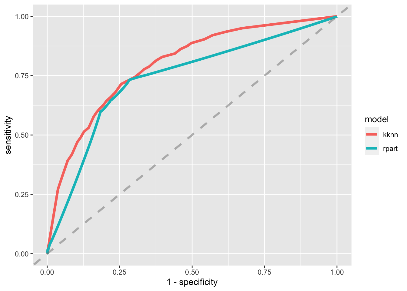
2 roc_auc  binary     0.742    25 0.00225 Preprocessor1_Model1

Code

knn_res %>%
  unnest(.predictions) %>%
  mutate(model = "kknn") %>%
  bind_rows(tree_res %>%
    unnest(.predictions) %>%
    mutate(model = "rpart")) %>%
  group_by(model) %>%
  roc_curve(children, .pred_children) %>%
  ggplot(aes(x = 1 - specificity, y = sensitivity, color = model)) +
  geom_line(size = 1.5) +
  geom_abline(
    lty = 2, alpha = 0.5,
    color = "gray50",
    size = 1.2
  )

Code

knn_conf <- knn_res %>%
  unnest(.predictions) %>%
  conf_mat(children, .pred_class)

knn_conf

          Truth
Prediction children none
  children     8077 2888
  none         3223 8412

Code

knn_conf %>%
  autoplot()

Code

#knn_fit %>%
#  predict(new_data = test_proc, type = "prob") %>%
#  mutate(truth = hotel_test$children) %>%
#  roc_auc(truth, .pred_children)

4 predictions

Code

predictions= knn_fit%>%
  predict(new_data = test_proc, type = "prob") %>%
  mutate(truth = hotel_test$children) 
 
head(predictions)  

# A tibble: 6 × 3
  .pred_children .pred_none truth   
           <dbl>      <dbl> <fct>   
1         0           1     none    
2         0.252       0.748 none    
3         0.775       0.225 children
4         0.0233      0.977 none    
5         0.0233      0.977 none    
6         0.0233      0.977 none    

Code

predictions %>%  roc_auc(truth, .pred_children)

# A tibble: 1 × 3
  .metric .estimator .estimate
  <chr>   <chr>          <dbl>
1 roc_auc binary         0.801

5 Reference

https://github.com/rfordatascience/tidytuesday/blob/master/data/2020/2020-02-11/readme.md

https://juliasilge.com/blog/hotels-recipes/

https://www.tidymodels.org/start/case-study/